 TFStudio
 Designing a Gain Flattening Filter for an Erbium Amplifier
Flatten a real erbium amplifier gain with a Ta2O5/SiO2 filter. Set the target from the gain or a loss curve, start from a thick seed, run Needle and Refinement.
Put the output of an erbium-doped fiber amplifier on an optical spectrum analyzer and the channels near 1531 nm stand several dB above the ones at 1550 nm, though every channel went in at the same power. After a few amplifiers in a chain the strong channels drown the weak ones. The usual fix sits inside the amplifier: a passive filter that loses exactly as much as the gain is too high. That is a gain flattening filter.
Its spectrum is easy to state and hard to build. Why does a filter that removes a few dB need to be about a tenth of a millimetre thick?
The gain curves
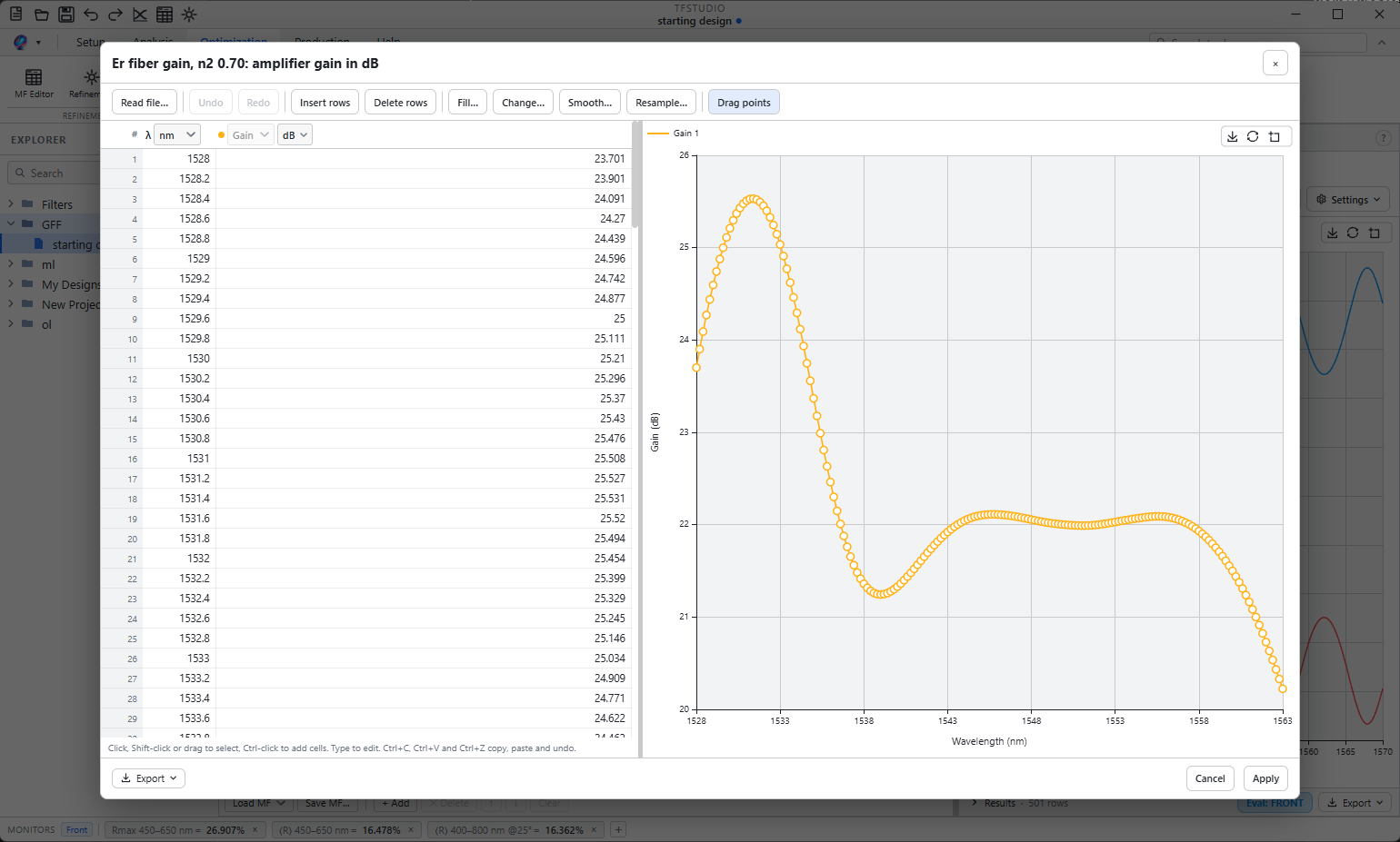
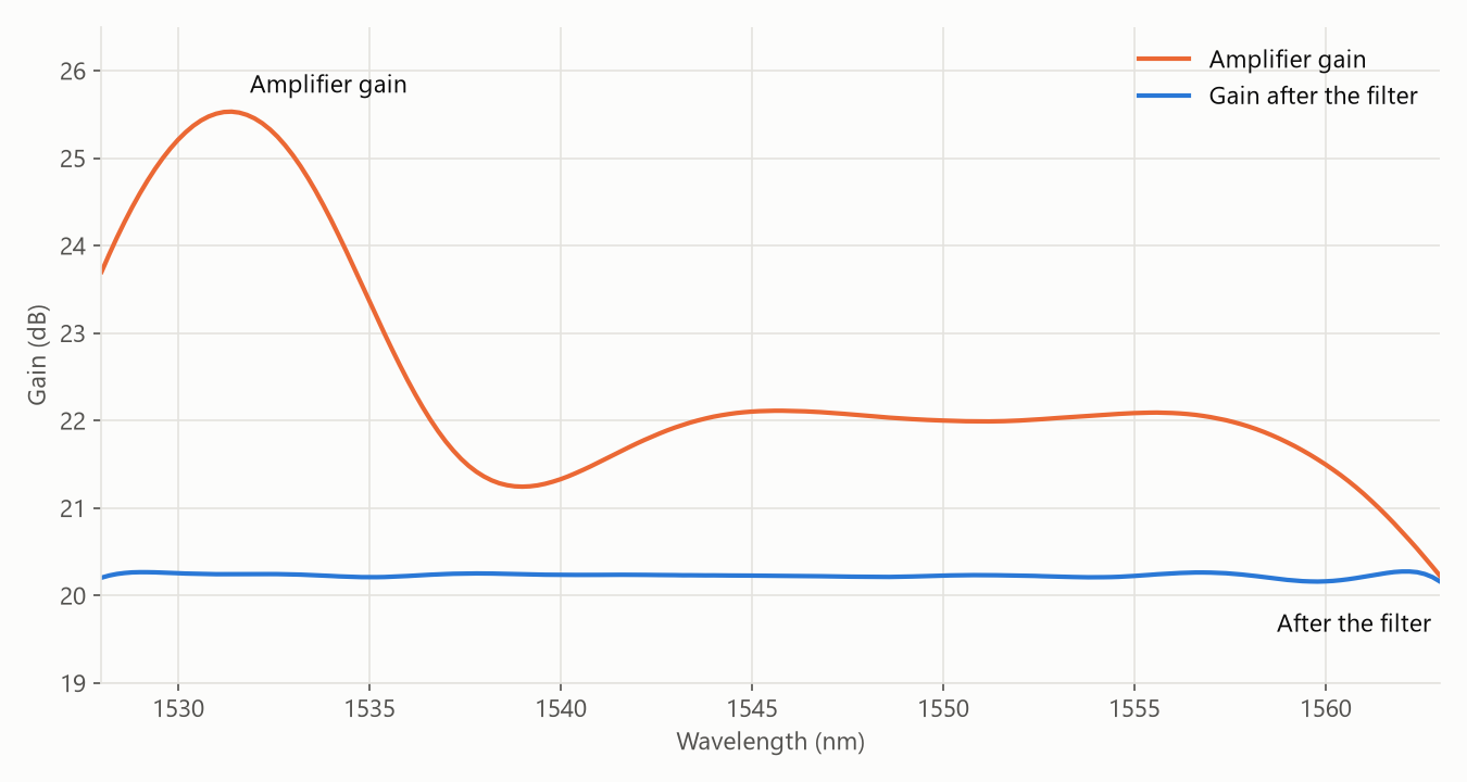
Both curves here are the gain of one real erbium-doped fiber, computed from its absorption and gain coefficients at two pump levels. The fiber data ships with OptiCommPy, an open-source optical communications simulator (GPL-3.0). For a fiber of length with a fraction of its erbium ions excited, averaged along the fiber, the gain in dB is
with the absorption and the gain coefficient, both in dB/m (Giles and Desurvire, J. Lightwave Technol. 9, 271, 1991).
| Gain file | Fiber length | Peak gain | Depth to flatten | |
|---|---|---|---|---|
| first curve | 0.70 | 10.7 m | 25.5 dB at 1531.4 nm | 5.3 dB |
| second curve | 0.75 | 9.1 m | 27.4 dB at 1531.0 nm | 7.7 dB |
Both files run from 1528 to 1563 nm. The fiber length is chosen so both give the same gain at 1550 nm, 22 dB. Pumping harder grows the 1531 nm peak, so the second filter has more to remove. This tutorial flattens the first curve and leaves the second as an exercise.
The design conditions:
- Band: 1528-1563 nm
- Incident medium: Air
- Substrate: SiO2 (fused silica)
- Coated surface: Front, with Ignore other side
- Angle of incidence: 0°, polarization Average
- Materials: Ta₂O₅ and SiO₂, no absorption at 1550 nm
- Goal: peak-to-peak error under 0.3 dB, the least insertion loss the coating can reach
What the filter has to do
A passive filter can only take light away, so it cannot lift the low parts of the gain. It brings every wavelength down to the lowest gain in the band:
That is 0 dB where the gain is lowest and negative everywhere else. The merit function wizard builds this target from the gain, or takes a target curve you already have.
Path A: you have the amplifier gain
Open the Merit Function Editor and fill in the wizard:
- Preset Curve target, type Gain flattening, input Amplifier gain (dB).
- Next to Gain, press Import… and pick the gain file.
- Press Type… to see what was read. It opens the curve editor on the gain, a table beside a plot.
- In the Angle and target box, leave Insertion loss and Peak-to-peak error at 0 dB. Zero asks for the best the coating can reach.
- Under Thickness limits, make sure the layer minimum is ticked and set it to 15 nm. Choosing Gain flattening unticks the layer maximum, because this filter needs thick layers.
- Press Generate.
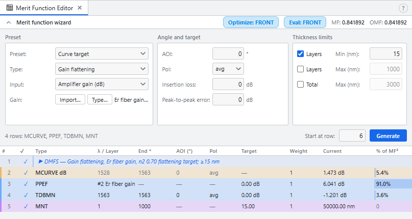
The wizard writes four rows:
| Row | What it scores |
|---|---|
MCURVE dB |
the shape: least squares between the design and the target, with a constant offset between them taken out |
PPEF |
peak-to-peak error: the highest less the lowest difference from the target, so a constant offset does not count. It is the number these filters are sold on |
TDBMN |
transmittance where the target is highest, kept no lower than 0 dB less the insertion loss |
MNT |
the 15 nm layer minimum |
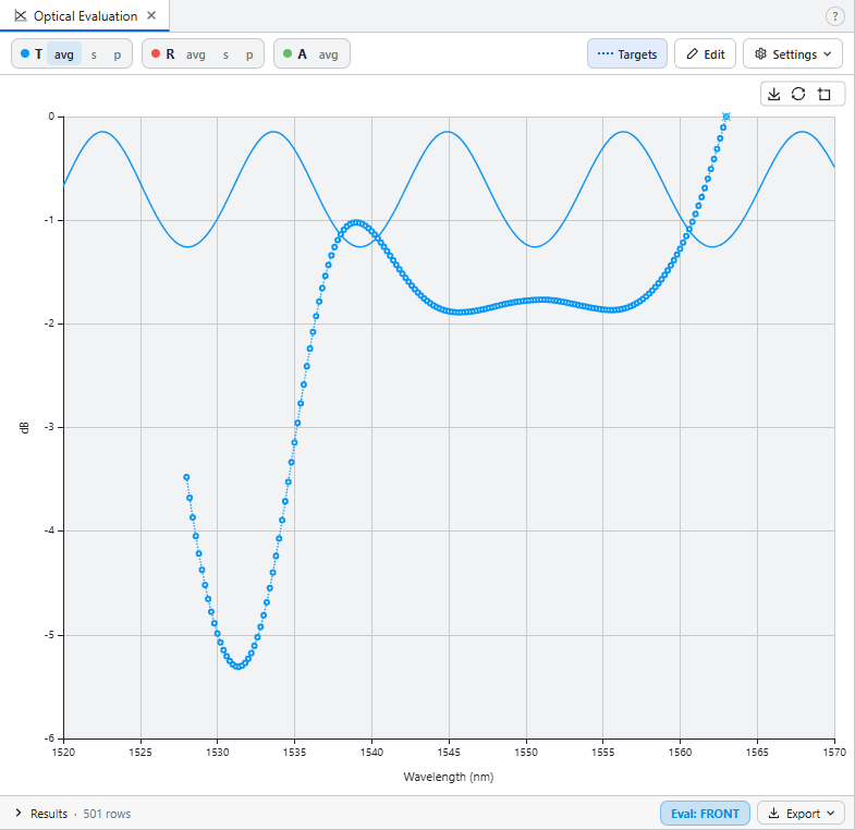
The target itself goes on the design as a transmittance curve named after the gain, so Optical Evaluation draws it over the spectrum.
Path B: you have the target loss curve
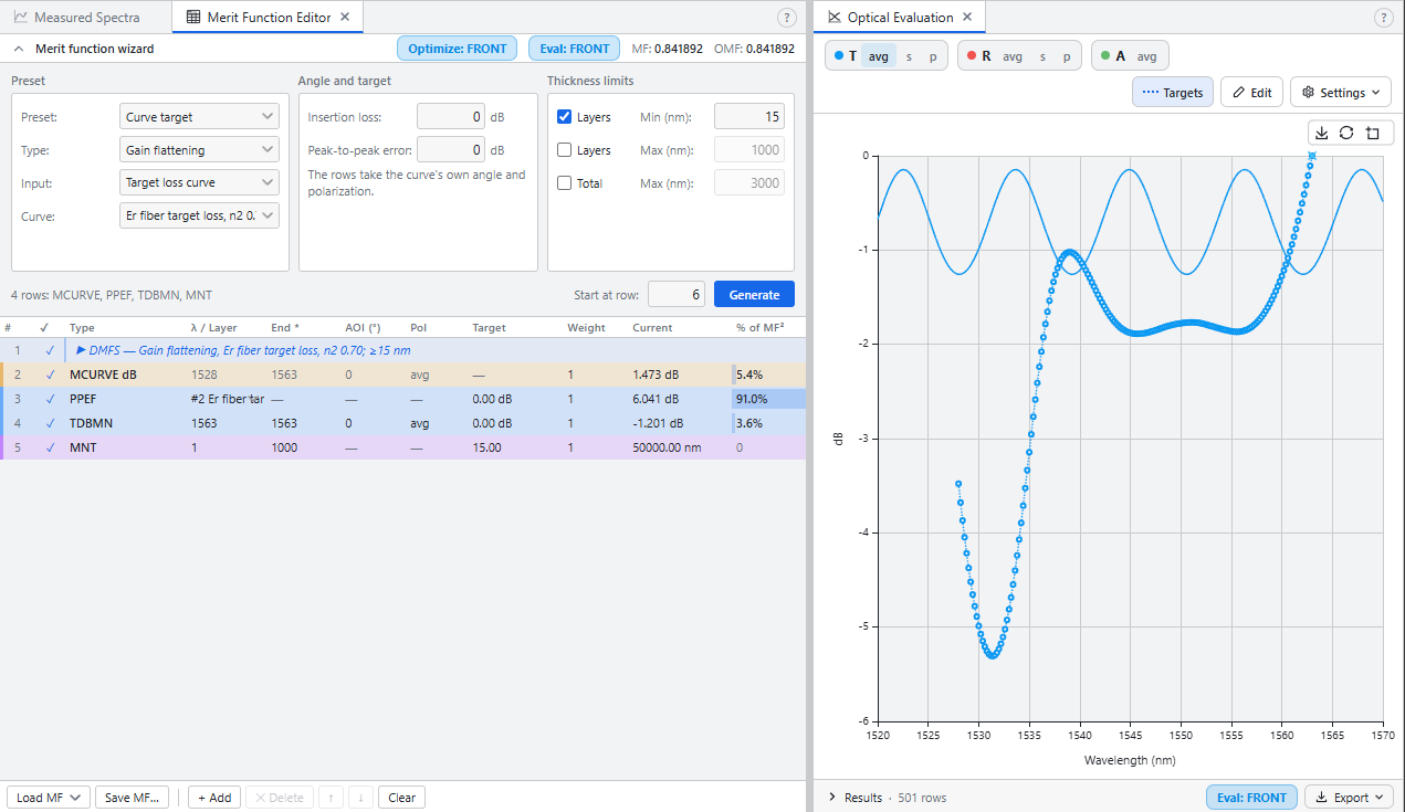
Sometimes the customer sends the filter's loss curve instead of the gain. To try this path, use the target for the first curve, written as positive attenuation the way a customer would send it. Bring it into Measured Spectra with New curve, then Read file… or paste, set the value column to T and its unit to dB loss, and Apply. That unit reads a loss as the positive number a customer writes; plain dB would read it as gain and mark every value as impossible.
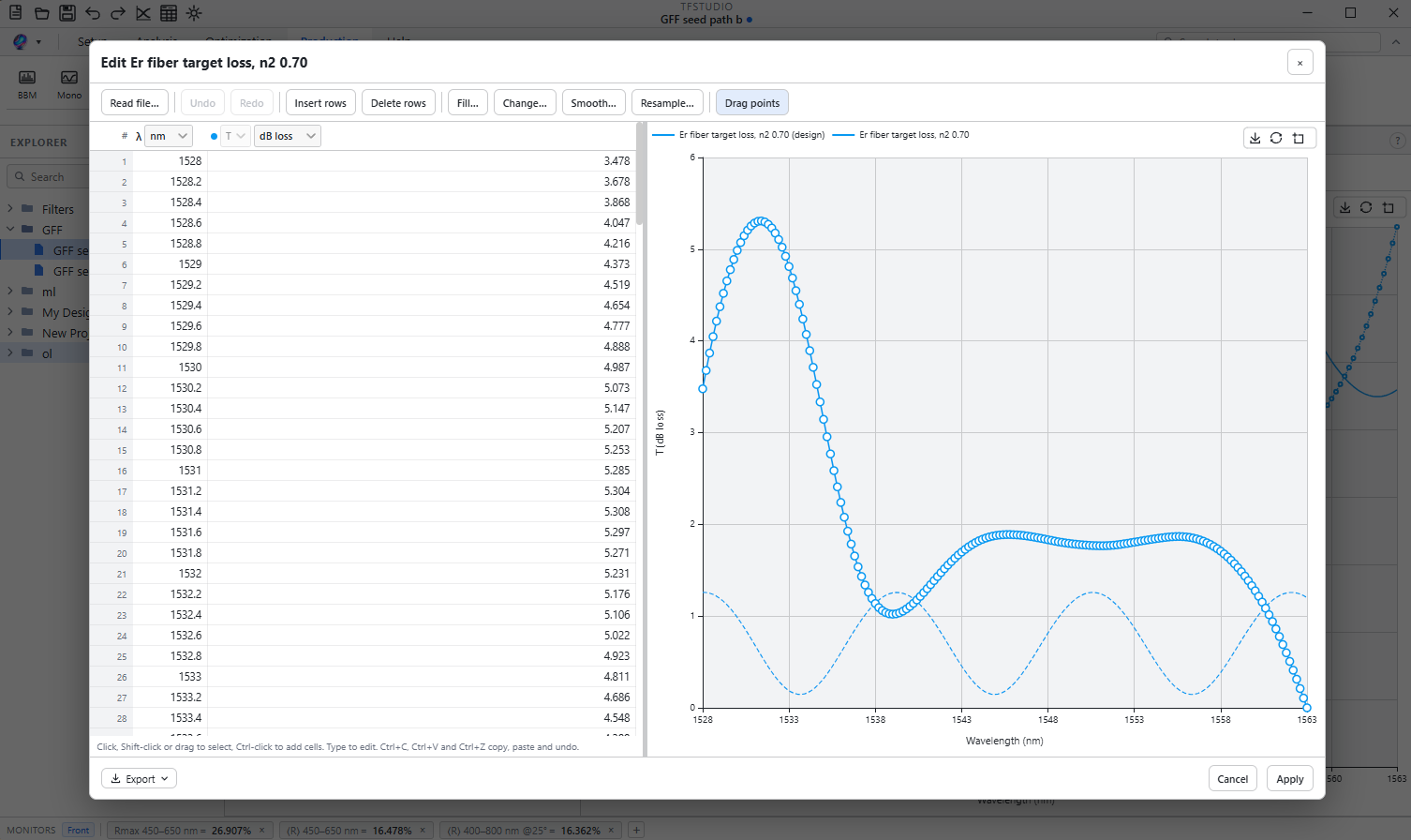
Then set the wizard's input to Target loss curve and pick the curve. With only one curve on the design, the wizard takes it without asking. Generate writes the same four rows.
Two lossless materials
| Material | Source | at 1550 nm | at 1550 nm |
|---|---|---|---|
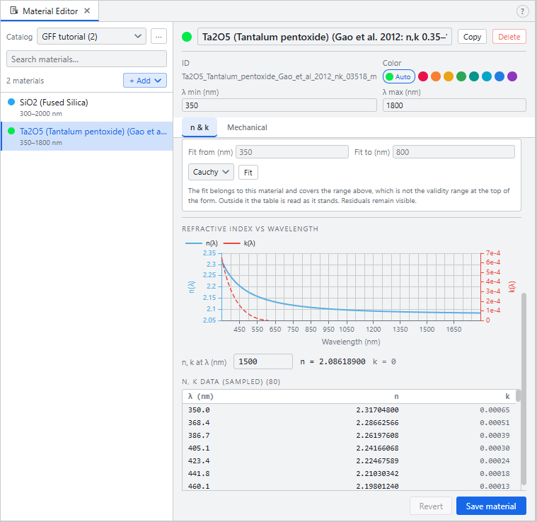
| Ta₂O₅ | refractiveindex.info, Gao et al. 2012, an ion-assisted e-beam film | 2.0856 | 0 |
| SiO₂ | built-in SiO2 (Fused Silica) |
1.4440 | 0 |
The built-in Ta2O5 is a different film, with at 1550 nm. That costs about 0.1 dB per micrometre of Ta₂O₅: harmless in a visible AR coating, several dB in this filter.
Put both materials in one catalog of their own. In the Material Editor, open ⋯, choose New empty catalog… and call it GFF tutorial. Then + Add → From refractiveindex.info…, find Ta2O5 → Gao et al. 2012 and add it to that catalog, where it is listed as Ta2O5 (Tantalum pentoxide) (Gao et al. 2012: n,k 0.35–1.8 µm). Last, select the built-in SiO2 (Fused Silica) and use Copy to my catalog….
Why the seed is a tenth of a millimetre thick
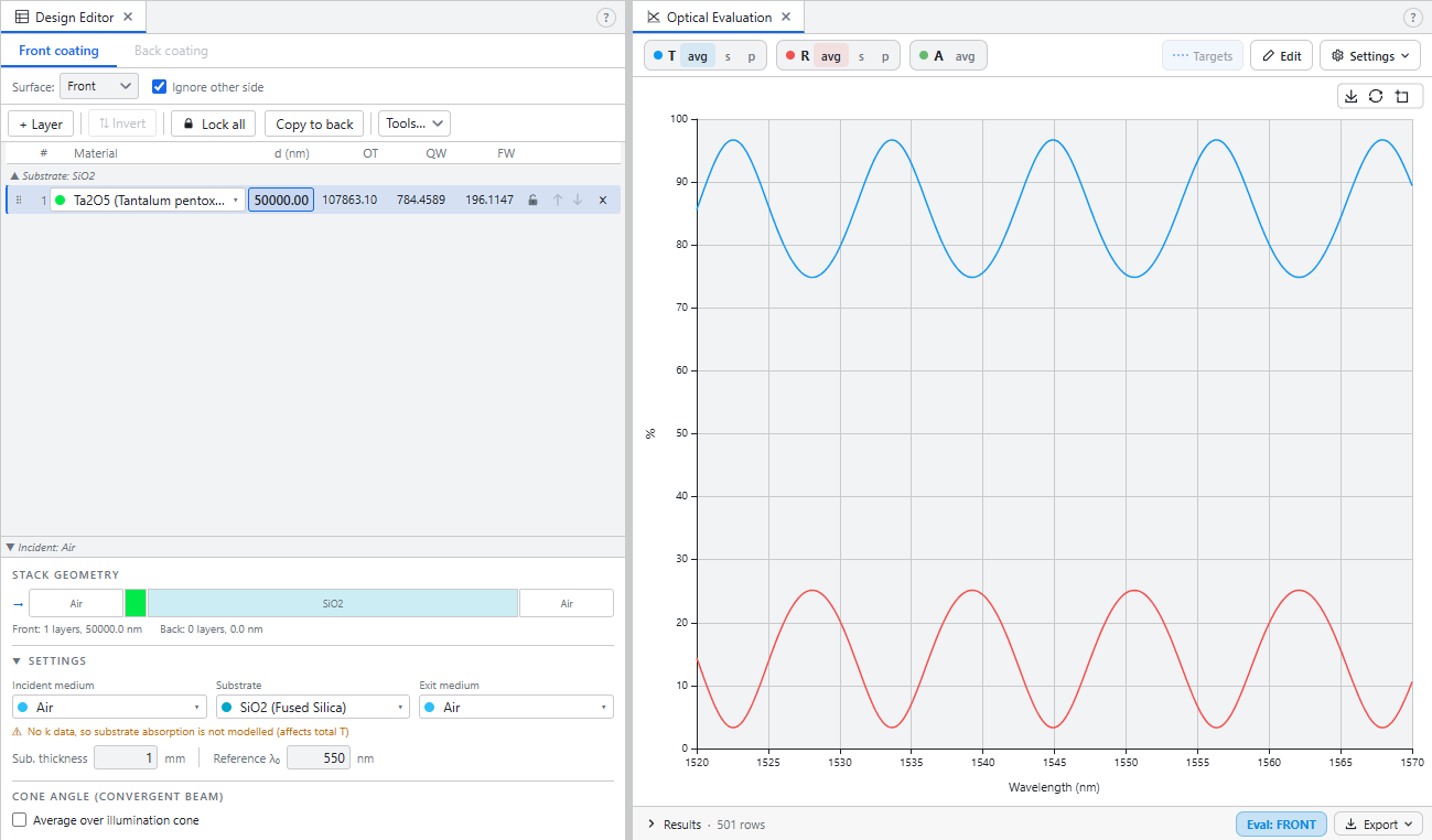
A coating's spectrum and its index profile are linked by a Fourier integral over twice the optical path (Macleod, Thin-Film Optical Filters, eq. 11.5). The practical reading: a stack cannot draw a spectral feature much narrower than , where is its total optical thickness. The 1531 nm peak is about 7 nm wide at half its height, so has to be of the order of nm, about 170 µm of optical path. In film, that is around a tenth of a millimetre.
Needle splits layers and moves material between them, but an insertion adds no thickness. Once per run, when it stalls, it restarts from a copy of the design two to sixteen times thicker. So the seed sets the scale and the restart fills in the rest:
| Design Editor layer | Material | Thickness |
|---|---|---|
| 1 | Ta2O5 (Gao), from GFF tutorial |
50,000 nm |
Step 1. Needle
Open Needle Automatic and set:
- Material Pool: tick the GFF tutorial catalog. The pool starts with the materials the design already uses, which here is only Ta₂O₅, and Needle needs SiO₂ to insert.
- Max layers: 60
The window notes that the PPEF row is left to Refinement. Needle puts each new layer where the merit function falls fastest, which is a derivative. The slope of a peak-to-peak error comes from just its two worst wavelengths, so with it on, every insertion chases those two points and the search stalls. The shape row gives a slope from every wavelength.
Press Run. The restart to a thicker copy shows as a Thicker start line in the history, and the run stops when no insertion lowers the merit any further.
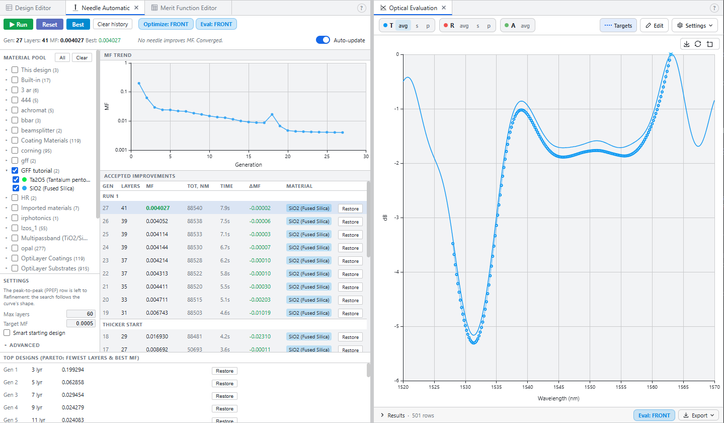
The design already follows the shape. It sits a little above the target through most of the band, which the shape row does not count, and meets it only at the long end, so the flattened gain dips there.
Step 2. Refinement
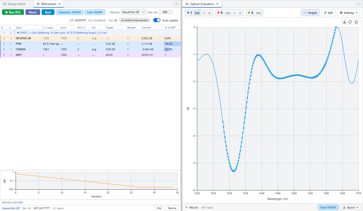
Before this step I raised the MNT row from 15 to 40 nm, for a thicker floor in the finished filter. Open Refinement and run Sequential QP. It works on every row, PPEF and the floor included, so it brings the worst points in and lifts every layer the needle left thinner than 40 nm.
The result
| Seed | After Needle | After Refinement | |
|---|---|---|---|
| Layers | 1 | 41 | 41 |
| Total thickness | 50.0 µm | 88.5 µm | 89.0 µm |
| Thinnest layer | 50.0 µm | 1.1 nm | 40.0 nm |
| Thickest layer | 50.0 µm | 16.3 µm | 16.4 µm |
| Peak-to-peak error | 6.04 dB | 0.24 dB | 0.12 dB |
| Insertion loss | 1.20 dB | 0.01 dB | 0.06 dB |
Refinement halved the peak-to-peak error and paid for it with a few hundredths of a dB of insertion loss: to pull the long end into line with the rest of the band, it lets slightly less light through where the target asks for all of it. The finished stack is about a tenth of a millimetre thick, as the Fourier estimate said it would be.
Angle, back face and deposition errors
The filter was designed at normal incidence for one coated surface. In a dual-fiber collimator package the beam meets it a degree or two off normal, which shifts the curve, and the design has to be made for that angle. The back face needs its own antireflection coating: bare fused silica reflects about 3.3%, which on its own is 0.15 dB of insertion loss.
A stack this thick with this many layers is also sensitive to deposition errors. How far the peak-to-peak error moves under thickness errors is the next question, and the Monte Carlo window answers it.
The second curve is a harder filter of the same kind. Flatten it with the same steps and compare how much thicker it comes out.